22 an introduction to networks
“No man is an island,
entire of itself;
every man is a piece of the continent,
a part of the main.”
-John Donne.
22.1 introduction
Networks are everywhere - they include, of course, the internet, which can be seen as a network of machines linked by cables and various cellular and satellite technologies. They also includes social network applications such as X and Instagram which operate within these networks. For engineers, networks are the structures that underlie power grids and transportation systems. For epidemiologists, networks describe the paths through which infectious diseases spread. For social scientists, networks are a key unit of analysis in understanding the structure of social groups. Phenomena as diverse as altruism (Apicella et al. 2012), kidney donations (Nikzad et al. 2021), and obesity (Christakis and Fowler 2007) can be understood, in part, as network phenomena. (That’s Christakis in the TED talk linked above).
Networks demand a different approach to data science: up ’til now, the building block of our projects have been data frames or tibbles - objects which can be represented by matrices of observations (rows) x variables (columns). Representing networks in this way is tricky, but we can represent a given network in this way.
In this chapter, we briefly introduce some key network concepts. We then consider how network structures can be examined and understood in the tidyverse. In the next chapter, we will consider a case study in network analysis, examining a bibliometric network structure of a scholarly discipline.
22.1.1 a simple example: networks and balance theory
Let’s begin by imagining that you have a friend - maybe you two are the last humans on the planet, or just might as well be. Then someone else comes along, and you don’t care for this person, but your friend does. We’ll represent this as an undirected, signed network consisting of just three nodes and the edges between them (Harary 1959).
# if you are running windows, these two lines
# will avoid warnings about missing fonts

#extrafont::font_import()
extrafont::loadfonts(device="win")
# Create a data frame for the nodes
nodes <- data.frame(
name = c("you", "best friend", "other person")
)
# Create a data frame for the edges
# The 'sign' column is used to represent positive (1) or negative (-1) relationships
edges <- data.frame(
from = c("you", "best friend", "you"),
to = c("best friend", "other person", "other person"), sign = c(1, 1, -1)
)
# Convert the data frames into a tidygraph object
# Use 'as_tbl_graph' to specify the node and edge data
triangle <- as_tbl_graph(edges, directed = FALSE) %>%
mutate(name = nodes$name)
# Visualize the imbalanced triangle
ggraph(triangle, layout = "circle") +
geom_edge_link(
aes(
color = factor(sign),
linetype = factor(sign)
),
arrow = NULL, # No arrows needed for undirected graph
width = 1.2 # Make edges more visible
) +
geom_node_point(size = 10, color = "green") +
geom_node_text(aes(label = name), repel = TRUE, size = 6) +
scale_edge_color_manual(
name = "Relationship",
values = c("1" = "blue", "-1" = "red"),
labels = c("1" = "Positive", "-1" = "Negative")
) +
scale_edge_linetype_manual(
name = "Relationship",
values = c("1" = "solid", "-1" = "dashed"),
labels = c("1" = "Positive", "-1" = "Negative")
) +
theme_graph() +
labs(
title = "Is three a bad number?" )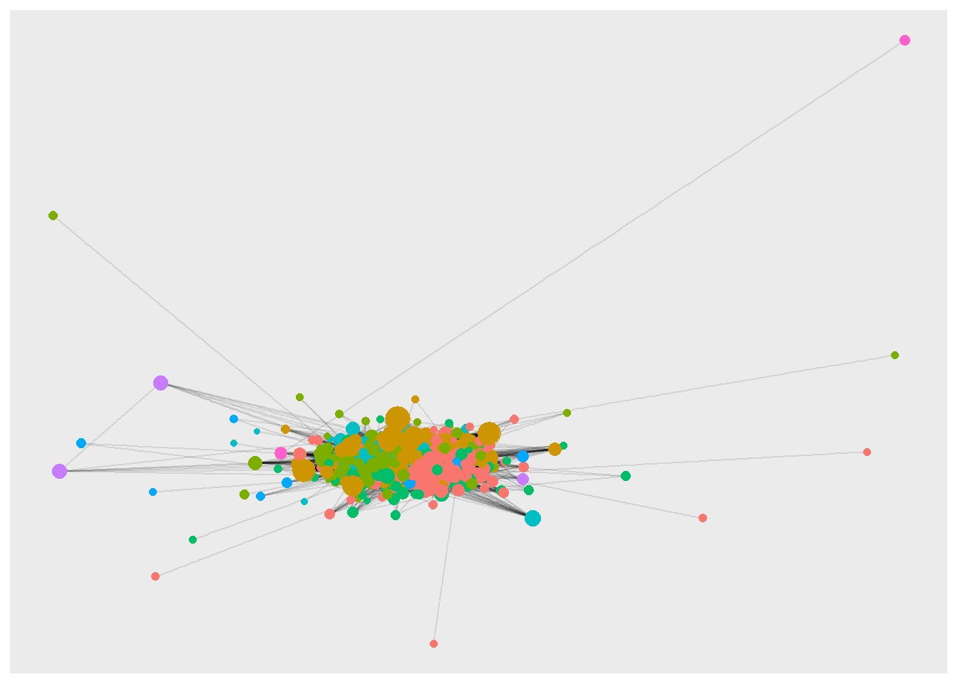
So. Is this system stable? What changes in edge weights might make it so? What changes would not make things better? What do all ‘stable’ (or ‘unstable’) networks have in common?
This is an application of balance theory (Cartwright and Harary 1956), which suggests that certain configurations of positive and negative edges are more stable than others. A recent NY Times article from a few years ago illustrates (kind of) how the complex geopolitical situation in the contemporary Middle East can be modeled using ideas drawn from balance theory and simple signed networks like the one above.
22.2 key network concepts
Networks involve two types of objects called nodes (or vertices) and edges (or links). Networks may be directed or undirected. Edges in a directed network might describe relationships such as likes, follows, has heard of, cites, or clicks on. We can represent them by arrows between nodes. Edges may be weighted. For example, in a network of a college curriculum, weights might correspond to the number of classes a student took with a particular professor.
Edges in an undirected network are symmetrical, as in the case of sharing a common property or ancestor. Undirected relationships are marked by phrases such as are siblings, are allies, know each other, are married, have been cited by the same source, and have both been exposed to. We can represent undirected networks by lines without arrowheads.
Unrequited love is a directed relationship, requited or reciprocal love can be modeled as undirected one.
Paths are series of connected edges between nodes.
Networks may be unsigned (only positive links) or signed (with positive and negative links).
In some networks, there is just one type of node. In addition to these single-mode networks, we will also encounter bipartite (two-mode) networks. A network of enrollments, for example, might include two types of nodes (e.g., classes and students). Edges in such a network describe relationships such as is enrolled in. In bipartite networks, there can only be links between different types of nodes (so classes can’t be enrolled in classes for example).
22.2.1 centrality
Within networks, nodes differ in centrality, connectedness, or importance. There are different measures and types of centrality - for example, the number (degree) of a node describes its number of connections. In directed networks, we can further distinguish between indegree centrality, for incoming links, and outdegree centrality, for outgoing ones. On some social media platforms, this might be described by ‘followers’ and ‘is following’, respectively.
Other measures of centrality gauge the importance of a node by the number of other nodes it connects (betweenness centrality). The most interesting measures of centrality, eigenvector centrality and PageRank, are recursive. That is, a node is central or important to the extent that the nodes to which it is linked are themselves central or important. PageRank was the original foundation of modern search engine on the Web. (The “Page” in PageRank does not refer to Webpage, but to Larry Page, one of the founders (with Sergey Brin) of Google (Page et al. 1999).
22.2.2 components and communities
Networks vary in their size (e.g., big vs small), number of discrete components (zero for the empty set, one for a network in which all nodes are directly or indirectly connected, more than this otherwise), and also in their community structure or clustering. Whereas the number of components in a network is relatively unambiguous, communities in networks are often fuzzy or difficult to discern, in much the same way that constellations in the night sky might seem arbitrarily ‘drawn.’
Just as there are many notions of centrality, there are also many approaches to thinking about communities. For example, we might use a “top-down” approach in which we begin with all of the nodes in a network and cleave them into two groups that both (a) minimize within-group distances and (b) maximize between-group distances. We could then repeat this strategy until we met some criterion. This approach gives a tree-like picture of community structure.
Alternatively, we can use a “bottom-up” approach to thinking about categories - combining the two closest nodes into a single community, then repeating this as appropriate. Communities in which all members are directly connected to all others are referred to as cliques. In the bottom-up approach, unlike the top-down approach, there are typically left-over nodes which are not connected to any community. In some applications of the bottom-up approach, communities are allowed to overlap, giving rise to complex structures such as that illustrated previously in Figure 20.1.
22.2.3 another example: it’s a small world
Consider a bipartite network in which there are two types of nodes, students and classes. An edge in this network represents a particular student who is enrolled in a particular class. Make a sketch of this network for you and a friend who is not in this class. Is there a path between the two of you? How about if we add another friend - or ten friends - to the network? What do we notice about the component structure of the network and the paths between nodes as the network grows bigger? (Milgram 1967).
In data science, it’s generally easiest to begin with very small datasets and to work towards bigger ones. With networks, this isn’t always the case, because very small networks may be structurally more complex than larger ones.
22.2.4 static and dynamic networks
Finally, we can distinguish between static networks (assessed at just one moment in time) and dynamic ones, which change. In dynamic networks, several important phenomena can be seen. One of these is contagion - not just of diseases, but also of emotions (Kelly, Iannone, and McCarty 2016) and a range of socially desirable and undesirable phenomena (Christakis and Fowler 2013). Another phenomena seen in dynamic networks is preferential attachment in which the most important nodes become still more important over time (Watts 2004).
Preferential attachment is reflected in many aspects of contemporary culture; we see it when a handful of restaurants or products ‘go viral’ while others struggle to attract customers. I believe that the acceleration of inequality of wealth and power in contemporary society is, in part, a product of the connectedness of the network in which we live, an unfortunate byproduct of efficient systems in the digital age.
ba <- play_barabasi_albert(n = 3, power = 1,
                           appeal_zero = 0, growth = 1,
                           directed = FALSE) |>
  ggraph(layout = "kk") +
  geom_node_point(aes(size = 1, color = "BLUE")) +
  geom_edge_link(alpha = 0.5) +
  theme_graph() +
  theme(legend.position = "none")
bb <- play_barabasi_albert(n = 10, power = 1,
                           appeal_zero = 0, growth = 1,
                           directed = FALSE) |>
  ggraph(layout = "kk") +
  geom_node_point(aes(size = 1, color = "BLUE")) +
  geom_edge_link(alpha = 0.5) +
  theme_graph() +
  theme(legend.position = "none")
bc <- play_barabasi_albert(n = 20, power = 1,
                           appeal_zero = 0, growth = 1,
                           directed = FALSE) |>
  ggraph(layout = "kk") +
  geom_node_point(aes(size = 1, color = "BLUE")) +
  geom_edge_link(alpha = 0.5) +
  theme_graph() +
  theme(legend.position = "none")
plot_grid (ba, bb, bc,
         nrow = 1, ncol = 3) +
  draw_figure_label("Preferential attachment: As networks grow, there is increasing inequality in centrality (degree)")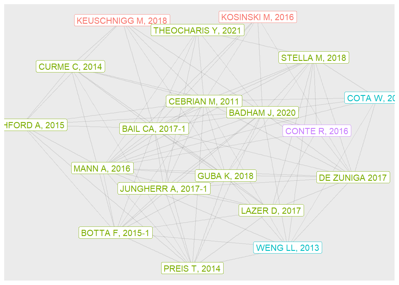
22.3 some additional sources
You can learn more about networks in the following resources:
Introduction to Networks with ggraph and The Simpsons
Intro to Network Analysis in R (Bail, SICSS)
Network chapter (Holster, Laboratory for Interdisciplinary Statistical Analysis). A comprehensive introduction and links to a case study of network psychometrics.
Bibliometric network videos (Lanning, see Chapter 23)
- CSSIntro0 GettingWOS Refs
- CSSIntro1 Citation and structural networks
- CSSIntro2 Visualizing networks
- CSSIntro3 Combining Text and Network analysis
#if needed, install.packages("")
library(tidyverse)
library(kableExtra) # for tables
library(bibliometrix) # for generating network from bib data & reducing to one mode
#library(qgraph)  # for drawing simple graphs
library(tidygraph) # for representing graphs as matrices of nodes/edges
library(igraph) # needed by tidygraph
library(ggraph)