25 exercises

25.1 generating correlated data (GPA and SAT) and putting it in a Google Sheet

It’s simple to generate a single random variable, but we often want to examine data for several variables that are correlated. The MVRnorm function, in the MASS package, does this.

We use this to generate two variables with mean 0 and standard deviation 1, a given correlation, and a given sample size (number of rows).

We then fiddle with these variables, setting the means, standard deviations, ranges, and number of significant digits, to make them look like GPA and SAT scores. And we use the randomnames package to make up fake names to go along with the fake scores. Finally, we upload the data to a Google Sheet. This last command will require first establishing permissions for R to read and write to your Google Drive.

knitr::opts_chunk$set(echo = TRUE)

library(tidyverse)
library(babynames) # for set of first names
library(randomNames) # for initial set of last names
library(googlesheets4) # to read and write to Google sheets

set.seed(33458) # for reproducibility
correlation <- 0.4
nrows <- 1000

names <- randomNames(nrows, which.names = "first") %>%
    bind_cols(randomNames(nrows, 
                          which.names = "last")) %>%
       rename (FirstName = 1, LastName = 2)

hsdata <- MASS::mvrnorm(n = nrows, 
                mu = c(0.0, 0),
                Sigma = matrix(
                    c(1, correlation, correlation, 1),
                    nrow = 2, ncol = 2)) %>% 
    as_tibble() %>%
    select (gpa = 1, sat = 2) %>% 
    mutate (sat = 500 + (100 * round(sat, 1))) %>% 
    mutate (gpa = 3 + round(gpa, 2)) %>%
    mutate (gpa = case_when(
        gpa < 0 ~ 0,
        gpa > 4.5 ~ 4.5,
        TRUE ~ gpa)) %>% 
    mutate (sat = case_when(
        sat < 200 ~ 200,
        gpa > 800 ~ 800,
        TRUE ~ sat))

hsdata <- names %>% 
    bind_cols(hsdata) %>% 
    arrange(FirstName) 
#gs4_create(name="RandomHSGPASAT",
 #          sheets = hsdata)
slice(hsdata, 1:3)

## # A tibble: 3 × 4
##   FirstName LastName    gpa   sat
##   <chr>     <chr>     <dbl> <dbl>
## 1 Aaliyah   Guttadore  0.72   510
## 2 Aaqil     Beltran    2.72   400
## 3 Aaqil     Robbe      0.75   400

25.1.1 now look at your data in the spreadsheet

In this spreadsheet, what are the means for GPA and SAT? What are the standard deviations? what is the difference between ‘sort range’ and ‘sort sheet’ in Google Sheets?

What do you think about the randomnames package? Do the names appear “representative” (of what)? If you wanted to generate a more representative sample of names, how might you proceed?

25.1.2 using AI to help us here

Our intuitions about the idiosyncratic nature of names in the randomNames package is supported (not necessarily confirmed) by MS Copilot, which notes that “the randomNames package in R samples from a uniform distribution, which doesn’t reflect real-world name frequencies.”

For first names, one solution is to use the babynames data, and then to weight the probability of including the name in our sample by the actual frequency in (some) population:

# load babynames and Filter for a specific year or range
names_data <- babynames %>%
  filter(year >= 2000) %>%
  group_by(name) %>%
  summarise(freq = sum(n)) %>%
  ungroup()

# Sample names with probability proportional to frequency
set.seed(33458)
sampled_first_names <- sample(names_data$name, size = nrows, replace = TRUE, prob = names_data$freq) |> 
    as_tibble() |> 
    rename(NewFirstName = 1)
slice(sampled_first_names, 1:10)

## # A tibble: 10 × 1
##    NewFirstName
##    <chr>       
##  1 Tea         
##  2 Emma        
##  3 Olivia      
##  4 Noemi       
##  5 Ruger       
##  6 Madelyn     
##  7 Jeffrey     
##  8 Caleb       
##  9 Audrey      
## 10 Elizabeth

25.1.3 for last names, it’s a little bit trickier

For last names, we’ll also use census data. There’s not an R package that has these, but there is Census data that is available in a zip file. It’s described at https://www2.census.gov/topics/genealogy/2010surnames/surnames.pdf. There are two files that are available - the top 1000 names, and then a (much longer) file of all names that occur more than 100 times. We’ll use the latter. Why do we do this?

Our approach to downloading a zip file directly into R follows: First, we specify a temporary file, then download the zip file into it. Then we unzip this and save it in a subdirectory called ‘data.’ Finally, we read it into R:

temp_zip_file <- tempfile(fileext = ".zip")
sourcefile <- "https://www2.census.gov/topics/genealogy/2010surnames/names.zip"
download.file(sourcefile, destfile = temp_zip_file, mode = "wb")
unzip(temp_zip_file, files = "Names_2010Census.csv", exdir = "data")
surnames <- read.csv("data/Names_2010Census.csv") |>
    arrange(rank)
slice(surnames, 1:10)

##               name rank    count prop100k cum_prop100k pctwhite pctblack pctapi pctaian pct2prace pcthispanic
## 1  ALL OTHER NAMES    0 29312001  9936.97      9936.97    66.65     8.53   7.97    0.86      2.32       13.67
## 2            SMITH    1  2442977   828.19       828.19     70.9    23.11    0.5    0.89      2.19         2.4
## 3          JOHNSON    2  1932812   655.24      1483.42    58.97    34.63   0.54    0.94      2.56        2.36
## 4         WILLIAMS    3  1625252   550.97      2034.39    45.75    47.68   0.46    0.82      2.81        2.49
## 5            BROWN    4  1437026   487.16      2521.56    57.95     35.6   0.51    0.87      2.55        2.52
## 6            JONES    5  1425470   483.24      3004.80    55.19    38.48   0.44       1      2.61        2.29
## 7           GARCIA    6  1166120   395.32      3400.12     5.38     0.45   1.41    0.47      0.26       92.03
## 8           MILLER    7  1161437   393.74      3793.86    84.11    10.76   0.54    0.66      1.77        2.17
## 9            DAVIS    8  1116357   378.45      4172.31     62.2     31.6   0.49    0.82      2.45        2.44
## 10       RODRIGUEZ    9  1094924   371.19      4543.50     4.75     0.54   0.57    0.18      0.18       93.77

25.1.4 cleaning these up

In the lastname data, there’s a problem. Some 10% of the names in the data - presumably rare ones - are replaced with “ALL OTHER NAMES.” We’ll just filter these out.

Finally, we combine the new NewFirstName and NewLastName with our original HS data. We also replace the SHOUTING (uppercase) in the NewLastName variable with Title Case:

Did we do this right? Any other issues? How might you have done this better?

surnames <- read.csv("data/Names_2010Census.csv") |>
    filter(name != "ALL OTHER NAMES")
slice(surnames, 1:10)

##         name rank   count prop100k cum_prop100k pctwhite pctblack pctapi pctaian pct2prace pcthispanic
## 1      SMITH    1 2442977   828.19       828.19     70.9    23.11    0.5    0.89      2.19         2.4
## 2    JOHNSON    2 1932812   655.24      1483.42    58.97    34.63   0.54    0.94      2.56        2.36
## 3   WILLIAMS    3 1625252   550.97      2034.39    45.75    47.68   0.46    0.82      2.81        2.49
## 4      BROWN    4 1437026   487.16      2521.56    57.95     35.6   0.51    0.87      2.55        2.52
## 5      JONES    5 1425470   483.24      3004.80    55.19    38.48   0.44       1      2.61        2.29
## 6     GARCIA    6 1166120   395.32      3400.12     5.38     0.45   1.41    0.47      0.26       92.03
## 7     MILLER    7 1161437   393.74      3793.86    84.11    10.76   0.54    0.66      1.77        2.17
## 8      DAVIS    8 1116357   378.45      4172.31     62.2     31.6   0.49    0.82      2.45        2.44
## 9  RODRIGUEZ    9 1094924   371.19      4543.50     4.75     0.54   0.57    0.18      0.18       93.77
## 10  MARTINEZ   10 1060159   359.40      4902.90     5.28     0.49    0.6    0.51      0.22       92.91

# then pull out a weighted sample of last names
sampled_last_names <- sample(surnames$name, size = nrows, 
                            replace = TRUE, prob = surnames$count) |> 
    as_tibble() |> 
    rename(NewLastName = 1)

hsdata2 <- hsdata |>
    bind_cols(sampled_first_names) |> 
    bind_cols(sampled_last_names) |> 
    mutate(NewLastName = stringr::str_to_title(NewLastName))
slice(hsdata2, 1:10)

## # A tibble: 10 × 6
##    FirstName LastName    gpa   sat NewFirstName NewLastName
##    <chr>     <chr>     <dbl> <dbl> <chr>        <chr>      
##  1 Aaliyah   Guttadore  0.72   510 Tea          Macdonald  
##  2 Aaqil     Beltran    2.72   400 Emma         Tornberg   
##  3 Aaqil     Robbe      0.75   400 Olivia       Pedraja    
##  4 Aaron     Taylor     3.93   470 Noemi        Carter     
##  5 Aaron     Baca       3.5    610 Ruger        Roberts    
##  6 Aaron     Johnston   2      360 Madelyn      Alicea     
##  7 Aasim     Warner     4.43   600 Jeffrey      Tucker     
##  8 Aasima    Kim        3.41   430 Caleb        Anderson   
##  9 Aasima    Lee        4.46   440 Audrey       Medina     
## 10 Aasiya    Dillard    3.57   450 Elizabeth    Vazquez

25.2 categorical probability and Venn diagrams

25.2.0.1 Dodge Chargers and FHP Cruisers

In 2024, the Florida Highway Patrol won a national competition for “best looking cruiser.” The winning car was a Dodge Charger.

Not all FHP cruisers are Dodge Chargers, but some are. Assume that there are 8 million registered cars in Florida, that all cars (including all FHP cruisers) are registered, and that 80,000 of these (or 1% of all cars) are Dodge Chargers.

1. On the basis of the above information, if you see a Dodge Charger on the road, can you compute the probability that it is an FHP cruiser (i.e., P(FHP cruiser | Dodge Charger)?

2. If you can compute this, what is the probability? If you cannot compute this, what is the minimum additional information would you need to compute this probability (P(FHP cruiser | Dodge Charger)?

3. Provide a reasonable estimate of this additional value, then compute (P(FHP cruiser | Dodge Charger).

4. Working with your own numbers, what is P(Dodge Charger | FHP cruiser)?

5. How confident are you in these results? Are there any additional assumptions that you might make that would make you more confident about your results?

Let A = P(FHP cruiser) B = P(Dodge Charger)

1. “not yet.”

2. Rule 4 gives us P(A|B) = P(A and B)/P(B)
   We have P(B) = .01 (80,000 / 8,000,000). We don’t have P(A and B): We need to know how many FHP Dodge Chargers there are out of the 8 million cars in Florida.

3. We will estimate the number of FHP Dodge Chargers as 800, or .0001 of the cars on the road.⁶
   So, P(A|B) = P(A and B)/P(B) = .0001/.01 = .01.
   That is, 1% of the Dodge Chargers on the road are FHP.

4. Here, we want the reverse probability P(B|A) [p(Dodge Charger | FHP cruiser)].
   We can use rule 4 again, just flipping around A and B:
   P(B|A) = P(A and B) / P(A) - but we first need to know the number of FHP Cruisers. This is the other missing number. We’ll estimate 1,600.⁷
   So P(A) = 1,600/8,000,000 = .0002
   So, P(B|A) = P(A and B)/P(A) = .0001/.0002 = .5.
   That is, half of 1% of the FHP cars on the road are Dodge Chargers.

5. Actually, we have been working with the number of registered cars - not the number that’s likely to be on the road at a given time. For this, FHP cruisers would need to be on the road with the same frequency as other vehicles - I’m guessing that they aren’t.

25.2.0.2 (Asymmetrical) Venn Diagrams in R

Problems about probability are often easier if we draw Venn diagrams.

1. Sketch out a Venn Diagram that accurately reflects the relationships you described in exercise 9.1.

2. Use R to generate your Venn Diagram.

3. Look at your figure. In general, if P(A|B) < P(B|A), what must be true of the relationship of P(A) to P(B)?

# Load required packages
library(VennDiagram)
library(grid)


# Create first Venn diagram
venn1 <- draw.pairwise.venn(
  area1 = 80000,
  area2 = 1600,
  cross.area = 800,
  category = c("Charger", "FHP"),
  fill = c("gray", "orange"),
  lty = "blank",
  cex = 1,#1.5,
  cat.cex = 1,
  cat.pos = c(-20, 40),
  cat.dist = 0.05,
  ind = FALSE
)

# To print Venn1, you need to wrap the figure using the grid package. The push and popViewport commands set the margins so it works right.
grid.newpage()
pushViewport(viewport(x = 0.5, y = 0.5, width = 0.9, height = 0.9))
grid.draw(venn1)
popViewport()

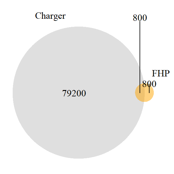
Here, P(A|B) is 800/1600 or .5, and P(B|A) is 800/80000 or .01.

If the base rate of A is greater than that of B, and there is at least some overlap, then P(A|B) > P(B|A).

---

6. Microsoft Copilot estimates this number as between 100 and 300. Claude estimates 800 to 1200. The midpoints of these are 200 and 1000; we’ll guess 800 (600 might be better, but 800 makes the math easier here, and we are really speculating).↩︎

7. Claude (“1,400-1,600”) and CoPilot (“several thousand”) are in relative agreement here.↩︎