18 cross-validation
The problem of capitalizing on chance is a significant one in prediction, and one should always be skeptical of models which are untested beyond the sample from which they were derived.
Here’s another dataset, the Fair (marital affairs) data, which is also included in the Ecdat package. You should read a little about it in the help window before proceeding.
To begin to examine univariate and bivariate relationships, we’ll apply ggpairs here, but for clarity will show only half of the data at a time. The dependent variable of interest (nbaffairs) will be included in both plots:
Fair1 <- Fair %>%
  select(sex:child, nbaffairs)
ggpairs(Fair1,
# if you wanted to jam all 9 vars onto one page you could do this
#        upper = list(continuous = wrap(ggally_cor, size = 10)),
         lower = list(continuous = 'smooth'),
         axisLabels = "none",
        switch = 'both')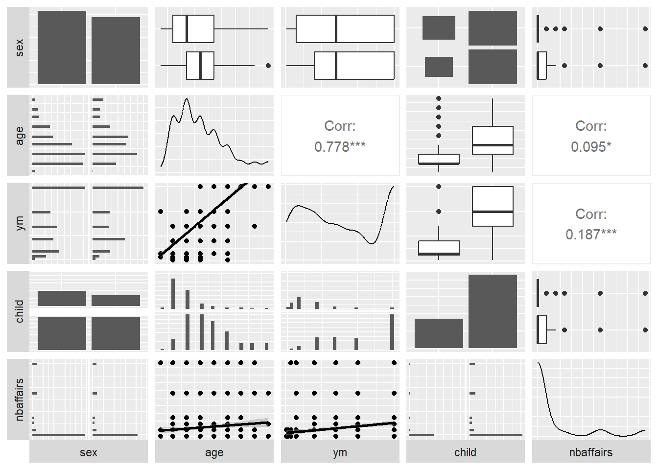
Fair2 <- Fair %>%
  select(religious:nbaffairs)
ggpairs(Fair2, lower = list(continuous = 'smooth'),
           axisLabels = "none",
           switch = 'both')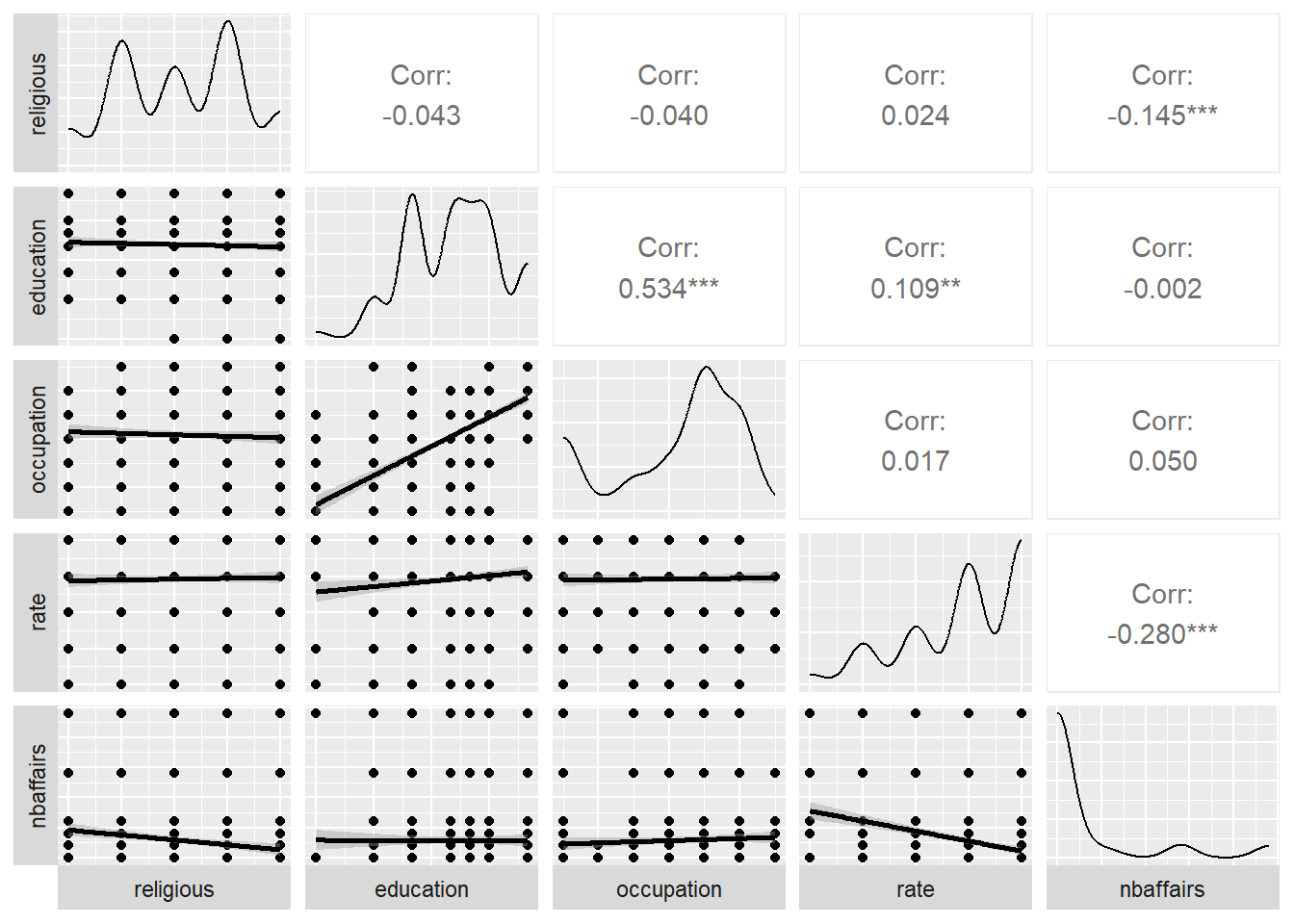
18.1 transformations
Look at the distribution of the “number of affairs” variable in the plots above. What does it look like?
##   nbaffairs   n
## 1         0 451
## 2         1  34
## 3         2  17
## 4         3  19
## 5         7  42
## 6        12  38
The distribution is skewed - and we realize that perhaps we should think about it differently: The meaning of the difference between 0 and 1 is not the same as that between 1 and 2, or perhaps even 1 and 12.
This suggests that perhaps we should transform the data. We might do this in several ways. We might perform a root transform, which we could then round to an integer:
##   rootAffair   n
## 1          0 451
## 2          1  70
## 3          2  42
## 4          3  38
Or we could simply distinguish between those that do and don’t have affairs.
##   affairYN   n
## 1        0 451
## 2        1 150
We’ll examine each of these in the following paragraphs.
18.2 avoiding capitalizing on chance
One lesson from the last class was that correlations (and regression coefficients) drawn from small samples were not stable. In regression analysis, as progressively smaller samples are drawn from a dataset, the ability to predict an outcome increases. In the limiting case, when the number of predictors (variables) is equal to the number of cases in the sample (rows), prediction became perfect. But if we were to apply the model to a new dataset, prediction would be poor.
18.2.1 splitting the data into training and test subsamples
The most basic solution to this problem is to split the data into two groups, a training sample from which we extract our model, and a test sample on which you will assess it. (Often, the logic of this will be extended to include a third group, a validation sample which would be used to tune or select the results of the training run before the test data are examined). Here, we will consider the simpler approach, splitting the Fair data into training and test samples. The critical feature of this analysis is that we will hold out the test data, and not even look at it until after our model building is complete.
# establish a seed for your data-split
# so that your results will be reproducible
set.seed(33458)
n <- nrow(Fair)
# create a set of line numbers
# of size corresponding to the
# desired training sample
trainIndex <- sample(1:n, size = round(0.6*n), replace=FALSE)
# create training and test samples
trainFair <- Fair[trainIndex ,]
testFair <- Fair[-trainIndex ,]
18.3 an example of cross-validated linear regression
We first predict the variable “rootAffair,” using just the training data:
trainFair2 <- trainFair %>%
    select(-nbaffairs, -affairYN)
testFair2 <- testFair %>%
    select(-nbaffairs, -affairYN)
model2 <- lm(rootAffair ~ ., data=trainFair2)
summary(model2)
##
## Call:
## lm(formula = rootAffair ~ ., data = trainFair2)
##
## Residuals:
## Min 1Q Median 3Q Max
## -1.6655 -0.4923 -0.2180 0.1444 2.7593
##
## Coefficients:
## Estimate Std. Error t value Pr(>|t|)
## (Intercept) 1.974758 0.385662 5.120 5.03e-07 ***
## sexmale -0.045067 0.106127 -0.425 0.6713
## age -0.014193 0.007835 -1.812 0.0709 .
## ym 0.038914 0.013901 2.799 0.0054 **
## childyes 0.027497 0.116926 0.235 0.8142
## religious -0.090619 0.038503 -2.354 0.0191 *
## education -0.018241 0.021963 -0.831 0.4068
## occupation 0.061293 0.030904 1.983 0.0481 *
## rate -0.265213 0.042161 -6.291 9.39e-10 ***
## ---
## Signif. codes: 0 '***' 0.001 '**' 0.01 '*' 0.05 '.' 0.1 ' ' 1
##
## Residual standard error: 0.8224 on 352 degrees of freedom
## Multiple R-squared: 0.1783, Adjusted R-squared: 0.1597
## F-statistic: 9.549 on 8 and 352 DF, p-value: 5.595e-12To assess the effectiveness of this model on an independent sample, we write a simple function, which assesses R2, then applies it to both the training data and the test data:
R2.model.dep.data <- function(myModel,myDep,myData) {
    errorscores <- myDep - predict(myModel,myData)
    SS.error <- sum(errorscores^2)
    deviations <- scale(myDep,scale = FALSE)#)
    SS.total <- sum(deviations^2)
    1 - (SS.error/SS.total)
}

(R2Train <- R2.model.dep.data(model2,trainFair2$rootAffair,trainFair2))
## [1] 0.1783303## [1] 0.003453435The R2 on the training sample is 0.1783303, on the test sample it is 0.0034534. The difference between these is sometimes referred to as shrinkage. Shrinkage will be problematic particularly when there are a small number of observations, a large number of predictors (and consequently a complex model), or both of these.
18.3.1 applying logistic regression analysis to the training data
Let’s go back to the “number of affairs” variable and consider a second way of thinking about it, that is, simply comparing those who do and don’t have affairs:
##   affairYN   n
## 1        0 451
## 2        1 150
With this change, the regression problem becomes more clearly a problem in classification. How can we best predict which ‘type’ (affair-ers vs. not) a given person falls in to?
With this change, we have moved from a variable which is essentially continuous (nbaffairs) to one which is dichotomous and therefore distributed binomially. The desired regression is now a logistic one.
We begin by running this analysis using only the training data.
##
## Call:
## glm(formula = affairYN ~ ., family = "binomial", data = trainFair)
##
## Coefficients:
##               Estimate Std. Error z value Pr(>|z|)
## (Intercept) -2.601e+01  1.434e+05   0.000    1.000
## sexmale      3.818e-02  3.891e+04   0.000    1.000
## age         -1.303e-02  3.176e+03   0.000    1.000
## ym           1.490e-02  5.403e+03   0.000    1.000
## childyes     2.288e-02  4.479e+04   0.000    1.000
## religious    2.225e-02  1.508e+04   0.000    1.000
## education    3.888e-02  8.532e+03   0.000    1.000
## occupation  -4.976e-02  1.113e+04   0.000    1.000
## rate        -1.357e-01  1.591e+04   0.000    1.000
## nbaffairs   -3.191e+01  4.714e+04  -0.001    0.999
## rootAffair   1.455e+02  1.626e+05   0.001    0.999
##
## (Dispersion parameter for binomial family taken to be 1)
##
##     Null deviance: 4.0981e+02  on 360  degrees of freedom
## Residual deviance: 3.2775e-09  on 350  degrees of freedom
## AIC: 22
##
## Number of Fisher Scoring iterations: 25
Examine your results. Is there a problem? If so, how do you fix it? When you have fixed it, how do you interpret the results?