25 exercises
25.2 categorical probability and Venn diagrams
25.2.0.1 Dodge Chargers and FHP Cruisers
In 2024, the Florida Highway Patrol won a national competition for “best looking cruiser.” The winning car was a Dodge Charger.

Not all FHP cruisers are Dodge Chargers, but some are. Assume that there are 8 million registered cars in Florida, that all cars (including all FHP cruisers) are registered, and that 80,000 of these (or 1% of all cars) are Dodge Chargers.
On the basis of the above information, if you see a Dodge Charger on the road, can you compute the probability that it is an FHP cruiser (i.e., P(FHP cruiser | Dodge Charger)?
If you can compute this, what is the probability? If you cannot compute this, what is the minimum additional information would you need to compute this probability (P(FHP cruiser | Dodge Charger)?
Provide a reasonable estimate of this additional value, then compute (P(FHP cruiser | Dodge Charger).
Working with your own numbers, what is P(Dodge Charger | FHP cruiser)?
How confident are you in these results? Are there any additional assumptions that you might make that would make you more confident about your results?
Let A = P(FHP cruiser) B = P(Dodge Charger)
“not yet.”
Rule 4 gives us P(A|B) = P(A and B)/P(B)
We have P(B) = .01 (80,000 / 8,000,000). We don’t have P(A and B): We need to know how many FHP Dodge Chargers there are out of the 8 million cars in Florida.We will estimate the number of FHP Dodge Chargers as 800, or .0001 of the cars on the road.6
So, P(A|B) = P(A and B)/P(B) = .0001/.01 = .01.
That is, 1% of the Dodge Chargers on the road are FHP.Here, we want the reverse probability P(B|A) [p(Dodge Charger | FHP cruiser)].
We can use rule 4 again, just flipping around A and B:
P(B|A) = P(A and B) / P(A) - but we first need to know the number of FHP Cruisers. This is the other missing number. We’ll estimate 1,600.7
So P(A) = 1,600/8,000,000 = .0002
So, P(B|A) = P(A and B)/P(A) = .0001/.0002 = .5.
That is, half of 1% of the FHP cars on the road are Dodge Chargers.Actually, we have been working with the number of registered cars - not the number that’s likely to be on the road at a given time. For this, FHP cruisers would need to be on the road with the same frequency as other vehicles - I’m guessing that they aren’t.
25.2.0.2 (Asymmetrical) Venn Diagrams in R
Problems about probability are often easier if we draw Venn diagrams.
Sketch out a Venn Diagram that accurately reflects the relationships you described in exercise 9.1.
Use R to generate your Venn Diagram.
Look at your figure. In general, if P(A|B) < P(B|A), what must be true of the relationship of P(A) to P(B)?
# Load required packages
library(VennDiagram)
library(grid)


# Create first Venn diagram
venn1 <- draw.pairwise.venn(
  area1 = 80000,
  area2 = 1600,
  cross.area = 800,
  category = c("Charger", "FHP"),
  fill = c("gray", "orange"),
  lty = "blank",
  cex = 1,#1.5,
  cat.cex = 1,
  cat.pos = c(-20, 40),
  cat.dist = 0.05,
  ind = FALSE
)

# To print Venn1, you need to wrap the figure using the grid package. The push and popViewport commands set the margins so it works right.
grid.newpage()
pushViewport(viewport(x = 0.5, y = 0.5, width = 0.9, height = 0.9))
grid.draw(venn1)
popViewport()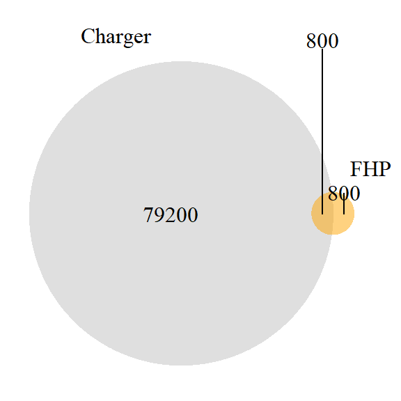
Here, P(A|B) is 800/1600 or .5, and P(B|A) is 800/80000 or .01.
If the base rate of A is greater than that of B, and there is at least some overlap, then P(A|B) > P(B|A).
Microsoft Copilot estimates this number as between 100 and 300. Claude estimates 800 to 1200. The midpoints of these are 200 and 1000; we’ll guess 800 (600 might be better, but 800 makes the math easier here, and we are really speculating).↩︎
Claude (“1,400-1,600”) and CoPilot (“several thousand”) are in relative agreement here.↩︎